NY HEAT Analysis

In [1]:

state_code = "NY"
state_fips = "36"
heat_cutoff = 0.06

NY HEAT and the Hudson Valley

In [2]:

library(tidyverse)

── Attaching core tidyverse packages ──────────────────────── tidyverse 2.0.0 ──
✔ dplyr     1.1.2     ✔ readr     2.1.4
✔ forcats   1.0.0     ✔ stringr   1.5.0
✔ ggplot2   3.4.2     ✔ tibble    3.2.1
✔ lubridate 1.9.2     ✔ tidyr     1.3.0
✔ purrr     1.0.1     
── Conflicts ────────────────────────────────────────── tidyverse_conflicts() ──
✖ dplyr::filter() masks stats::filter()
✖ dplyr::lag()    masks stats::lag()
ℹ Use the conflicted package (<http://conflicted.r-lib.org/>) to force all conflicts to become errors

library(sf)

Linking to GEOS 3.10.2, GDAL 3.4.1, PROJ 8.2.1; sf_use_s2() is TRUE

library(gt)
library(tigris)

To enable caching of data, set `options(tigris_use_cache = TRUE)`
in your R script or .Rprofile.

library(sf)
library(tidycensus)
options(tigris_use_cache=TRUE, tigris_year=2019)

In [3]:

hudson_valley <- tribble(
  ~county, ~region, ~fips,
  "Westchester", "Lower Hudson Valley", 36119,
  "Rockland", "Lower Hudson Valley", 36087,
  "Putnam", "Lower Hudson Valley", 36115,
  "Orange", "Mid-Hudson Valley", 36121,
  "Dutchess", "Mid-Hudson Valley", 36027,
  "Ulster", "Mid-Hudson Valley", 36111,
  "Sullivan", "Upper Hudson Valley", 36053,
  "Columbia", "Upper Hudson Valley", 36021,
  "Greene", "Upper Hudson Valley", 36017,
  "Albany", "Upper Hudson Valley", 36001,
  "Rensselaer", "Upper Hudson Valley", 36083
)

In [4]:

puma_county_mapping <- read_csv("/mnt/data/buildings2/geocorr/puma_county_mapping.csv", skip=1) |>
  janitor::clean_names()

Rows: 187 Columns: 9
── Column specification ────────────────────────────────────────────────────────
Delimiter: ","
chr (4): PUMA (2012), State abbr., County name, PUMA12 name
dbl (5): State code, County code, Total housing units (2020 Census), county-...

ℹ Use `spec()` to retrieve the full column specification for this data.
ℹ Specify the column types or set `show_col_types = FALSE` to quiet this message.

In [5]:

vars <- c("BLD", "PUMA", "HFL", "TEN", "YRBLT", "HINCP", "NP", "MV", "BDSP", "ELEP", "FULP", "GASP", "MRGP", "RNTP", "RMSP", "ELEFP", "FULFP", "GASFP")

# Get data from the Census API
filename <- paste0("/mnt/data/pums_1_22_", state_fips, ".Rds")

# Get data from the Census API
if (file.exists(filename)) {
  raw_data <- readRDS(filename)
} else {
  raw_data <- get_pums(variables = vars,
                 state = state_fips,
                 year = 2022,
                 survey = "acs1",
                 rep_weights = "housing",
                 recode = TRUE) |>
          distinct(SERIALNO, .keep_all = TRUE) # housing units only, not people
  saveRDS(raw_data, filename)
}

In [6]:

county_lmi <- readxl::read_excel("/mnt/data/buildings2/HUD_2021_income_limits_by_NY_county.xlsx") |>
  pivot_longer(-County, names_to = "NP") |>
  rename(lmi_cutoff = value)

In [7]:

data <- raw_data |>
  filter(HINCP != -60000) |> # remove missing for now
  mutate(HINCP = HINCP+1,
   bill_in_rent = (ELEFP == "1") | (GASFP == "1") | (FULP == "1"),
    GASP = case_when(
    GASP <= 4 ~ 0,
    .default = GASP
  ),
   ELEP = case_when(
    ELEP <= 3 ~ 0,
    .default = ELEP
  ),
   FULP = case_when(
    FULP <= 3 ~ 0,
    .default = FULP
   ),
  yearly_energy_bill = (ELEP + GASP) * 12 + FULP,
  energy_burden_pct = yearly_energy_bill / (HINCP+1),
  monthly_energy_burden = (yearly_energy_bill - (heat_cutoff*HINCP))/12,
  is_energy_burdened = energy_burden_pct > heat_cutoff,
  # `utility` bill does not include delivered fuel
  yearly_utility_bill = (ELEP + GASP) * 12,
  utility_burden_pct = yearly_utility_bill / (HINCP+1),
  monthly_utility_burden = (yearly_utility_bill - (heat_cutoff*HINCP))/12,
  is_utility_burdened = utility_burden_pct > heat_cutoff) |>
  inner_join(puma_county_mapping, by = c("PUMA" = "puma_2012"),
            relationship = 'many-to-many') |>
  inner_join(hudson_valley, by = c('county_code' = 'fips')) |>
  mutate(wt = WGTP * puma12_to_county_allocation_factor) |>
  mutate(NP = as.character(NP)) |>
  inner_join(county_lmi, by = c("county" = "County", "NP")) |>
  mutate(is_lmi = HINCP <= lmi_cutoff)

In [8]:

total_rollup <- data |>
  filter(!bill_in_rent) |>
  summarise(
    households_included = sum(wt),
    median_income = DescTools::Median(HINCP, weights = wt),
    pct_energy_burdened = weighted.mean(is_energy_burdened, w = wt),
    pct_utility_burdened = weighted.mean(is_utility_burdened, w =wt),
    avg_monthly_bill_of_burdened = weighted.mean(case_when(
      is_energy_burdened ~ yearly_energy_bill/12), w = wt,
      na.rm = TRUE),
    utility_burden_of_burdened = mean(case_when(
      is_utility_burdened ~ monthly_utility_burden), w = wt,
      na.rm = TRUE)) |>
mutate(county = "All",
      region = "Hudson Valley")

In [9]:

county_rollup <- data |>
  filter(!bill_in_rent) |>
  summarise(
    households_included = sum(wt),
    median_income = DescTools::Median(HINCP, weights = wt),
    pct_energy_burdened = weighted.mean(is_energy_burdened, w = wt),
    pct_utility_burdened = weighted.mean(is_utility_burdened, w =wt),
    avg_monthly_bill_of_burdened = weighted.mean(case_when(
      is_energy_burdened ~ yearly_energy_bill/12), w = wt,
      na.rm = TRUE),
    utility_burden_of_burdened = mean(case_when(
      is_utility_burdened ~ monthly_utility_burden), w = wt,
      na.rm = TRUE),
    .by = county) |>
  left_join(hudson_valley, by = "county") |>
  select(-fips)

In [10]:

total_rollup$pct_energy_burdened[[1]] |> scales::percent(1)

[1] "24%"

In [11]:

bind_rows(total_rollup, county_rollup) |>
  select(region, county, pct_energy_burdened, avg_monthly_bill_of_burdened, utility_burden_of_burdened) |>
  group_by(region) |>
  gt() |>
  row_group_order(c("Hudson Valley", "Upper Hudson Valley", "Mid-Hudson Valley", "Lower Hudson Valley")) |>
  fmt_currency(c(avg_monthly_bill_of_burdened,
    utility_burden_of_burdened), decimals = 0) |>
  fmt_percent(c(pct_energy_burdened), decimals = 0) |>
  cols_label(
    county = "County",
    pct_energy_burdened = "Energy Burdened Households (%)",
    avg_monthly_bill_of_burdened = "Avg. Monthly Energy Bills of Burdened Households",
    utility_burden_of_burdened = "Avg. Monthly Savings Under NY HEAT for Burdened Households",
  ) |>
  tab_header("NY HEAT in the Hudson Valley", subtitle = "Household energy burdens and savings by county") |>
  tab_footnote("Excluding households with utility bills in rent, or missing fuel or income information.\nSource: 2022 ACS. Win Climate, 2024")

NY HEAT in the Hudson Valley
Household energy burdens and savings by county
County	Energy Burdened Households (%)	Avg. Monthly Energy Bills of Burdened Households	Avg. Monthly Savings Under NY HEAT for Burdened Households
Hudson Valley
All	24%	$348	$148
Upper Hudson Valley
Albany	19%	$255	$117
Greene	35%	$318	$136
Rensselaer	23%	$287	$119
Columbia	32%	$319	$140
Sullivan	28%	$294	$131
Mid-Hudson Valley
Dutchess	25%	$338	$138
Ulster	32%	$340	$144
Orange	27%	$269	$111
Lower Hudson Valley
Rockland	27%	$389	$192
Putnam	29%	$288	$116
Westchester	21%	$404	$183
Excluding households with utility bills in rent, or missing fuel or income information. Source: 2022 ACS. Win Climate, 2024

In [12]:

county_rollup |>
  summarise(sum(utility_burden_of_burdened * households_included))

# A tibble: 1 × 1
  `sum(utility_burden_of_burdened * households_included)`
                                                    <dbl>
1                                              131845967.

In [13]:

data |>
  filter(!is.na(is_lmi)) |>
  group_by(is_lmi) |>
  summarise(pct_energy_burdened = weighted.mean(is_energy_burdened, w = wt))

# A tibble: 2 × 2
  is_lmi pct_energy_burdened
  <lgl>                <dbl>
1 FALSE               0.0507
2 TRUE                0.458 

In [14]:

county_boundaries <- counties("NY")

Retrieving data for the year 2019

county_boundaries |>
  right_join(county_rollup, by = c("NAME" = "county")) |>
  mutate(label = paste0(NAME," (", scales::percent(pct_energy_burdened, 1) ,")")) |>
  ggplot(aes(fill=pct_energy_burdened, label=label)) +
  geom_sf(color = "black") +
  ggrepel::geom_label_repel(
    aes(geometry = geometry),
    fill = "white",
    stat = "sf_coordinates",
    min.segment.length = 0
    ) +
  scale_fill_distiller(palette = "Spectral",
                       name = "Percentage",
                       limits = c(0, .5),
                       labels = scales::percent_format(scale=100)) +
  theme_void() +
  labs(title = "Energy Burden by County",
       subtitle = "Win Climate, 2024\n(Source: 2022 ACS)",
       pct = "Percent")

Warning in st_point_on_surface.sfc(sf::st_zm(x)): st_point_on_surface may not
give correct results for longitude/latitude data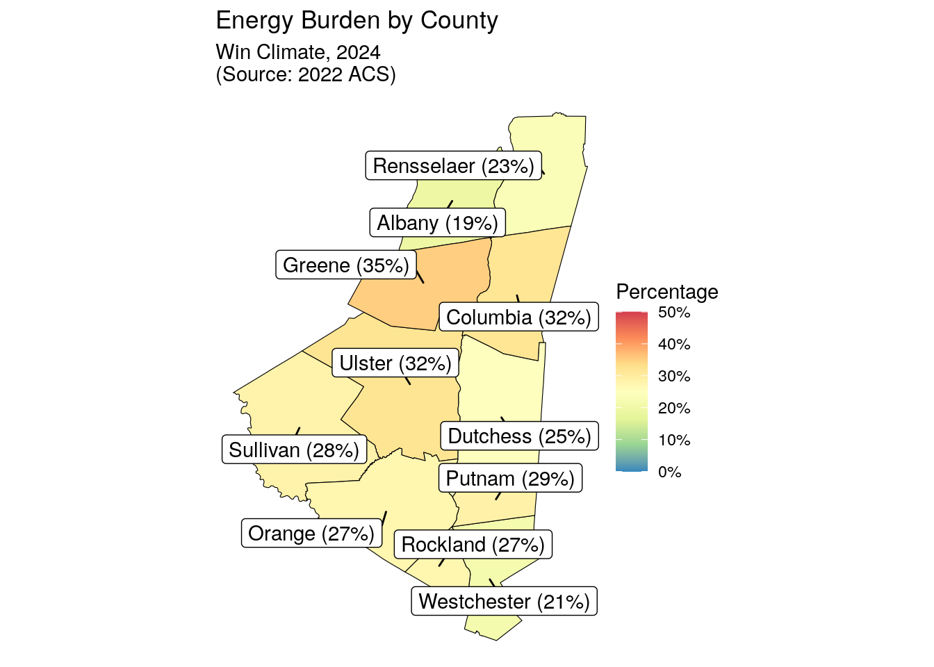

In [15]:

county_boundaries |>
  right_join(county_rollup, by = c("NAME" = "county")) |>
  mutate(label = paste0(NAME," (", scales::dollar(utility_burden_of_burdened, 1) ,")")) |>
  ggplot(aes(fill=utility_burden_of_burdened, label=label)) +
  geom_sf(color = "black") +
  ggrepel::geom_label_repel(
    aes(geometry = geometry),
    fill = "white",
    stat = "sf_coordinates",
    min.segment.length = 0
    ) +
  scale_fill_distiller(palette = "Greens",
                       direction = 1,
                       name = "NY HEAT Savings",
                       labels = scales::dollar_format(accuracy = 1),
                       limits = c(0, 250)) +
  theme_void() +
  labs(title = "Average Monthly NY HEAT Savings by County",
       subtitle = "Win Climate, 2024\n(Source: 2022 ACS)")

Warning in st_point_on_surface.sfc(sf::st_zm(x)): st_point_on_surface may not
give correct results for longitude/latitude data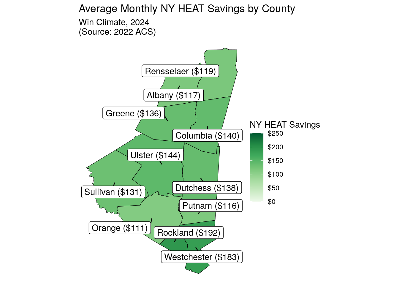

In [16]:

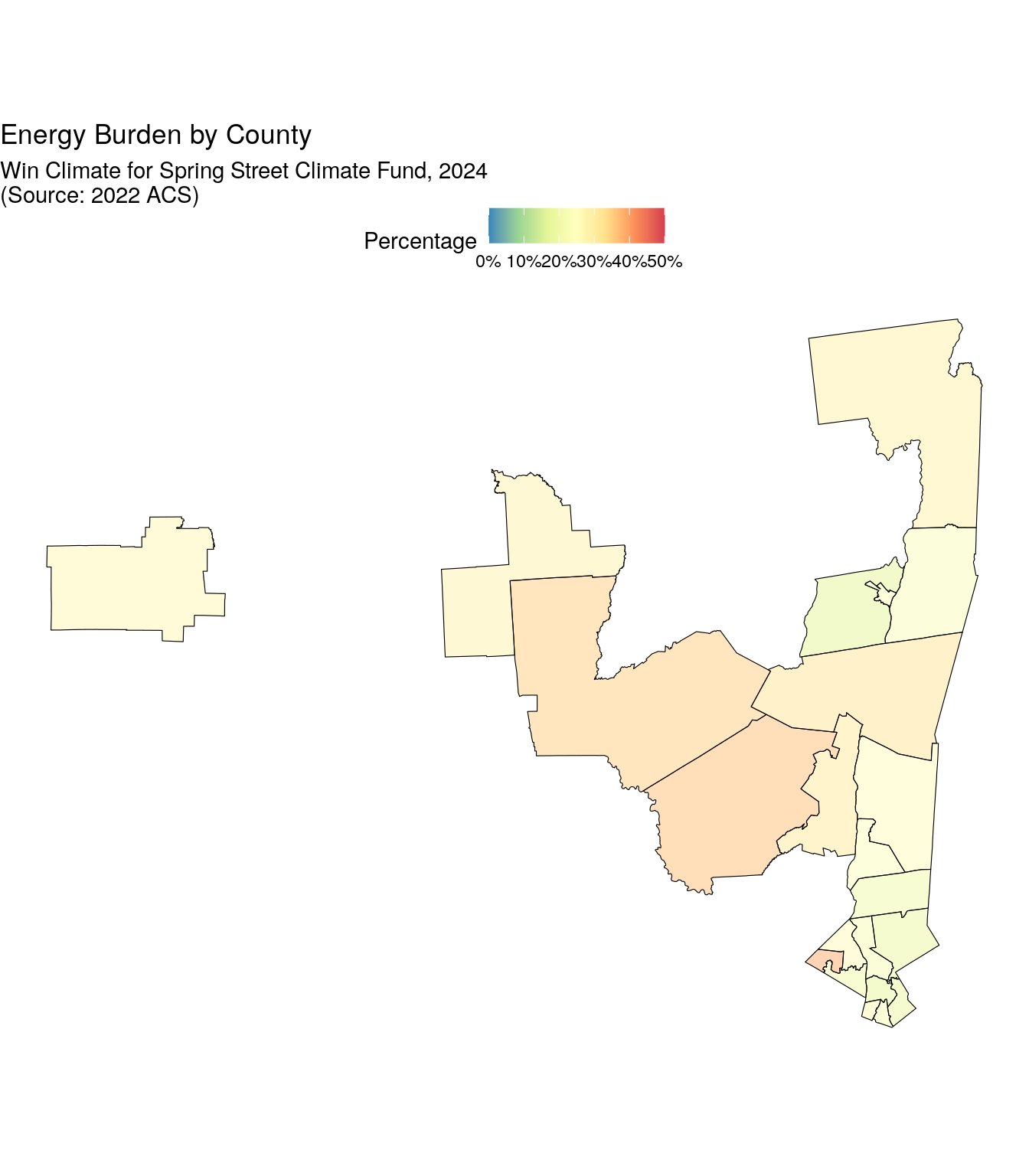
puma_boundaries <- pumas("NY", 2019)

Retrieving data for the year 2019

puma_rollup <- data |>
  filter(!bill_in_rent) |>
  summarise(
    households_included = sum(wt),
    median_income = DescTools::Median(HINCP, weights = wt),
    pct_energy_burdened = weighted.mean(is_energy_burdened, w = wt),
    avg_monthly_bill_of_burdened = weighted.mean(case_when(
      is_energy_burdened ~ yearly_energy_bill/12), w = wt,
      na.rm = TRUE),
    utility_burden_of_burdened = mean(case_when(
      is_energy_burdened ~ monthly_energy_burden), w = wt,
      na.rm = TRUE),
    .by = c(puma12_name, PUMA))  |>
  mutate(GEOID10 = paste0(state_fips, PUMA))

puma_boundaries |>
  right_join(puma_rollup, by = c("GEOID10")) |>
  #mutate(label = paste0(NAME," (", scales::percent(pct_energy_burdened, 1) ,")")) |>
  ggplot(aes(fill=pct_energy_burdened)) +#, label=label)) +
  geom_sf(color = "black", alpha=.5) +
  #ggrepel::geom_label_repel(
  #  aes(geometry = geometry),
  #  fill = "white",
  #  stat = "sf_coordinates",
  #  min.segment.length = 0
  #  ) +
  scale_fill_distiller(palette = "Spectral",
                       name = "Percentage",
                       limits = c(0, .5),
                       labels = scales::percent_format(scale=100)) +
  theme_void() +
  theme(legend.position = "top") +
  labs(title = "Energy Burden by County",
       subtitle = "Win Climate for Spring Street Climate Fund, 2024\n(Source: 2022 ACS)",
       pct = "Percent")